Barycentric coordinate system (mathematics)
In geometry, the barycentric coordinate system is a coordinate system in which the location of a point is specified as the center of mass, or barycenter, of masses placed at the vertices of a simplex (a triangle, tetrahedron, etc). Barycentric coordinates are a form of homogeneous coordinates. The system was introduced (1827) by August Ferdinand Möbius.
Contents |
Definition
Let  be the vertices of a simplex in a vector space A. If, for some point
  in A,
in A,

and at least one of  does not vanish then we say that the coefficients () are barycentric coordinates of with respect to . The vertices themselves have the coordinates
  . Barycentric coordinates are not unique: for any b not equal to zero, (
 ) are also barycentric coordinates of p.
When the coordinates are not negative, the point lies in the convex hull of , that is, in the simplex which has those points as its vertices.
Barycentric coordinates on triangles
In the context of a triangle, barycentric coordinates are also known as areal coordinates, because the coordinates of P with respect to triangle ABC are proportional to the (signed) areas of PBC, PCA and PAB. Areal and trilinear coordinates are used for similar purposes in geometry.
Barycentric or areal coordinates are extremely useful in engineering applications involving triangular subdomains. These make analytic integrals often easier to evaluate, and Gaussian quadrature tables are often presented in terms of area coordinates.
First let us consider a triangle T defined by three vertices  ,
,  and
and  . Any point
  located on this triangle may then be written as a weighted sum of these three vertices, i.e.
where  ,
,  and
and  are the area coordinates (usually denoted as

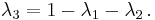
 ). These are subjected to the constraint
which means that
Following this, the integral of a function  on T is

Note that the above has the form of a linear interpolation. Indeed, area coordinates will also allow us to perform a linear interpolation at all points in the triangle if the values of the function are known at the vertices.
Converting to barycentric coordinates
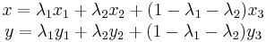
Given a point  inside a triangle it is also desirable to obtain the barycentric coordinates , and at this point. We can write the barycentric expansion of vector having Cartesian coordinates
  in terms of the components of the triangle vertices (
 ,
,  ,
,  ) as
) as
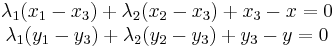
substituting  into the above gives
Rearranging, this is
This linear transformation may be written more succinctly as
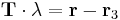
Where  is the vector of barycentric coordinates, is the vector of Cartesian coordinates, and
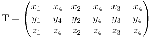
  is a matrix given by
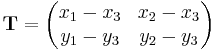
Now the matrix is invertible, since  and
and  are linearly independent (if this were not the case, then , , and would be collinear and would not form a triangle). Thus, we can rearrange the above equation to get
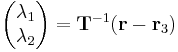
Finding the barycentric coordinates has thus been reduced to finding the inverse matrix of , an easy problem in the case of 2×2 matrices.
Explicitly, the formulae for the barycentric co-ordinates of  are:
are:


Determining if a point is inside a triangle
Since barycentric coordinates are a linear transformation of Cartesian coordinates, it follows that they vary linearly along the edges and over the area of the triangle. If a point lies in the interior of the triangle, all of the Barycentric coordinates lie in the open interval  . If a point lies on an edge of the triangle, at least one of the area coordinates
  is zero, while the rest lie in the closed interval
 ![[0,1]](/2012-wikipedia_en_all_nopic_01_2012/I/ccfcd347d0bf65dc77afe01a3306a96b.png) .
.
Summarizing,
- Point lies inside the triangle if and only if
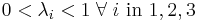 .
. - Otherwise, lies on the edge or corner of the triangle if
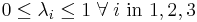 .
. - Otherwise, lies outside the triangle.
Interpolation on a triangular unstructured grid
Barycentric coordinates provide a convenient way to interpolate a function on an unstructured grid or mesh, as long as the function's value is known at all vertices of the mesh.
To interpolate a function  at a point , we go through each triangular element and transform into the barycentric coordinates of that triangle. If , then the point lies in the triangle or on its edge (explained in the previous section). Now, we interpolate the value of as

This linear interpolation is automatically normalized since  .
.
Barycentric coordinates on tetrahedra
Barycentric coordinates may be easily extended to three dimensions. The 3D simplex is a tetrahedron, a polyhedron having four triangular faces and four vertices. Once again, the barycentric coordinates are defined so that the first vertex maps to barycentric coordinates  ,
,  , etc.
This is again a linear transformation, and we may extend the above procedure for triangles to find the barycentric coordinates of a point with respect to a tetrahedron:
where  is now a 3×3 matrix:
Once again, the problem of finding the barycentric coordinates has been reduced to inverting a 3×3 matrix. 3D barycentric coordinates may be used to decide if a point lies inside a tetrahedral volume, and to interpolate a function within a tetrahedral mesh, in an analogous manner to the 2D procedure. Tetrahedral meshes are often used in finite element analysis because the use of barycentric coordinates can greatly simplify 3D interpolation.
Generalized barycentric coordinates
Barycentric coordinates (a1, ..., an) that are defined with respect to a polytope instead of a simplex are called generalized barycentric coordinates. For these, the equation

is still required to hold where x1, ..., xn are the vertices of the given polytope. Thus, the definition is formally unchanged but while a simplex with n vertices needs to be embedded in a vector space of dimension of at least n-1, a polytope may be embedded in a vector space of lower dimension. The simplest example is a quadrilateral in the plane. Consequently, even normalized generalized barycentric coordinates (i.e. coordinates such that the sum of the coefficients is 1) are in general not uniquely determined anymore while this is the case for normalized barycentric coordinates with respect to a simplex.
More abstractly, generalized barycentric coordinates express a polytope with n vertices, regardless of dimension, as the image of the standard  -simplex, which has n vertices – the map is onto:
  The map is one-to-one if and only if the polytope is a simplex, in which case the map is an isomorphism; this corresponds to a point not having unique generalized barycentric coordinates.
Dual to generalized barycentric coordinates are slack variables, which measure by how much margin a point satisfies the linear constraints, and gives an embedding 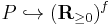 into the f-orthant, where f is the number of faces (dual to the vertices). This map is one-to-one (slack variables are uniquely determined) but not onto (not all combinations can be realized).
This use of the standard -simplex and f-orthant as standard objects that map to a polytope or that a polytope maps into should be contrasted with the use of the standard vector space  as the standard object for vector spaces, and the standard affine hyperplane
 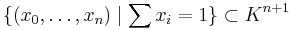 as the standard object for affine spaces, where in each case choosing a linear basis or affine basis provides an isomorphism, allowing all vector spaces and affine spaces to be thought of in terms of these standard spaces, rather than an onto or one-to-one map (not every polytope is a simplex). Further, the n-orthant is the standard object that maps to cones.
Applications
Generalized barycentric coordinates have applications in computer graphics and more specifically in geometric modelling. Often, a three-dimensional model can be approximated by a polyhedron such that the generalized barycentric coordinates with respect to that polyhedron have a geometric meaning. In this way, the processing of the model can be simplified by using these meaningful coordinates.
See also
References
- Bradley, Christopher J. (2007). The Algebra of Geometry: Cartesian, Areal and Projective Co-ordinates. Bath: Highperception. ISBN 978-1-906338-00-8.
- Weisstein, Eric W., "Areal Coordinates" from MathWorld.
- Weisstein, Eric W., "Barycentric Coordinates" from MathWorld.
External links
- The uses of homogeneous barycentric coordinates in plane euclidean geometry
- Barycentric Coordinates – a collection of scientific papers about (generalized) barycentric coordinates
- Barycentric coordinates: A Curious Application (solving the "three glasses" problem) at cut-the-knot
- Point in triangle test